7. Functional analysis
Sequedex not only places each 10-mer on a phylogenetic tree, but it also searches an 962 example sets of genes for a functional assignment as well. For the seed_0911.m1 set of functional assignments, we used the SEED classification of functions, which have the added benefit of a well-defined hierarchical rollup. The names and sets of genes are ennumerated in section Definition of functional classifications, where clicking on each label provides the annotation for each gene included (across the phylogeny) in the subsystem. For the ribosome, category si_0962, both the large and small subunits from across the 1550 species in the tree of life were translated into all three forward reading frames to make 10-mer ‘amino acid’ signatures, while the bacteria and archaea also had the tRNAs translated in a similar fasion. In the event a gene with a 10-mer signature appears in multiple categories, a metagenomic read contains 10-mers from different genes in different categories, the read is apportioned equally among all categories.
In additional to the genomic (DNA) metagenomic data sets with the phylogenetic profiles examined in the previous chapter:
- the set of
synthetic data from reference genomeswithlabels, - a set of
environmental microbiomeswithlabels - a set of
human microbiomeswithlabels
we provide transcriptomic (RNA) data sets from publically available data sets to illustrate the comparisons:
- a set of
human tisue-specific expressionwithlabels - a set of
marine eukaryotic transcriptomeswithlabels - a set of
transcriptomes from plaque microbiomeswithlabels
7.1. Visualizing SEED functional profiles with Sequestat
Graphical visualization can occur with Sequestat and the igraph package in R. You will first need to download the functional definitions (or use any what-Life2550-xxGB.0xseed_0911.m1.tsv file). Here, we assume both it and sequestat.r are available in the user’s home directory (~/), and that the working directory of the R session is in a directory containing sequedex output files. Also, we assume the user is using the .Rdata file with the graph layout in it. Since we often do not want Ribosomal or Unclassified read counts to skew normalizations when plotting counts, we set them to zero. Analysis of all of the data sets will start with the following:
source("~/Sequedex-docs/dl/sequestat.r")
library(igraph)
load("~/Sequedex-docs/dl/seed.layout.Rdata")
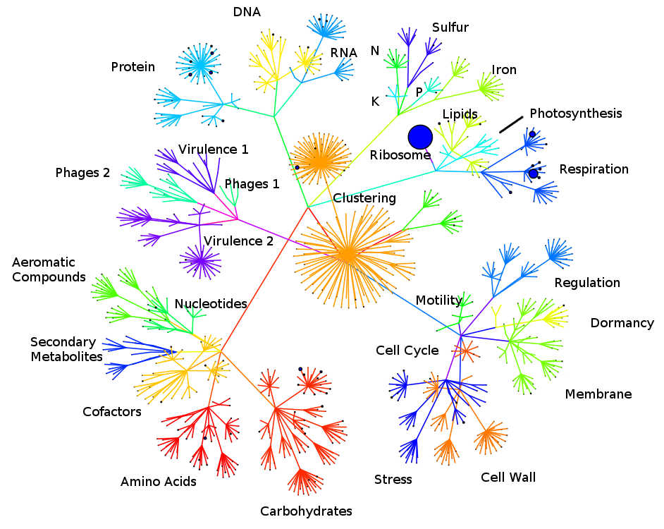
This results in the graph layout below, to which we have added labels to aid in reading the graphs below, from which we leave the labels off.
Reading in particular Sequedex output files will begin with:
expt <- Read.functional("./", "~/Sequedex-docs/dl/what", type.ref="Life2550-40", data.type="what")
expt$layout=seed.layout
expt$data[963,]=0
expt$data[964,]=0
plot.graph(hatlas,1, simple.name= T,scol= "blue",sign= F, dimension= 2,cex=0.6)
To read in the tsv data sets listed above, download them and read them into the data structures as follows:
source("~/Sequedex-docs/dl/sequestat.r")
library(igraph)

syn=Read.graph("~/Sequedex-docs/dl/what", col=TRUE, sat=1)
data=read.table("~/Sequedex-docs/dl/syn.Life.what",sep="\t",header=F)
syn$data=data
load("~/seed.layout.Rdata")
syn$layout=seed.layout
syn$data[963,]=0
lbl=read.table("~/Sequedex-docs/dl/syn.Life.lbl",sep="\t",header=F)
lbl=lbl[!is.na(lbl)]
colnames(syn$data)=lbl
plot.graph(syn,1, simple.name= F,scol= "blue",sign= T, dimension= 2,cex=0.6)
Diff.graph(syn,1,2, dim=2, alpha= 0.000000001)

env=Read.graph("~/Sequedex-docs/dl/what", col=TRUE, sat=1)
data=read.table("~/Sequedex-docs/dl/env.Life.what",sep="\t",header=F)
env$data=data
load("~/seed.layout.Rdata")
env$layout=seed.layout
env$data[963,]=0
lbl=read.table("~/Sequedex-docs/dl/env.Life.lbl",sep="\t",header=F)
lbl=lbl[!is.na(lbl)]
colnames(env$data)=lbl
plot.graph(env,1, simple.name= F,scol= "blue",sign= T, dimension= 2,cex=0.6)
Diff.graph(env,1,2, dim=2, alpha= 0.000000001)

hmb=Read.graph("~/Sequedex-docs/dl/what", col=TRUE, sat=1)
data=read.table("~/Sequedex-docs/dl/hmb.Life.what",sep="\t",header=F)
hmb$data=data
load("~/seed.layout.Rdata")
hmb$layout=seed.layout
hmb$data[963,]=0
lbl=read.table("~/Sequedex-docs/dl/hmb.Life.lbl",sep="\t",header=F)
lbl=lbl[!is.na(lbl)]
colnames(hmb$data)=lbl
plot.graph(hmb,1, simple.name= F,scol= "blue",sign= T, dimension= 2,cex=0.6)
Diff.graph(hmb,1,2, dim=2, alpha= 0.000000001)

hatlas=Read.graph("~/Sequedex-docs/dl/what", col=TRUE, sat=1)
data=read.table("~/Sequedex-docs/dl/hatlas.Life.what",sep="\t",header=F)
hatlas$data=data
load("~/seed.layout.Rdata")
hatlas$layout=seed.layout
hatlas$data[963,]=0
lbl=read.table("~/Sequedex-docs/dl/hatlas.Life.lbl",sep="\t",header=F)
lbl=lbl[!is.na(lbl)]
colnames(hatlas$data)=lbl
plot.graph(hatlas,1, simple.name= F,scol= "blue",sign= T, dimension= 2,cex=0.6)
Diff.graph(hatlas,1,2, dim=2, alpha= 0.000000001)

ocean=Read.graph("~/Sequedex-docs/dl/what", col=TRUE, sat=1)
data=read.table("~/Sequedex-docs/dl/ocean.Life.what",sep="\t",header=F)
ocean$data=data
load("~/seed.layout.Rdata")
ocean$layout=seed.layout
ocean$data[963,]=0
lbl=read.table("~/Sequedex-docs/dl/ocean.Life.lbl",sep="\t",header=F)
lbl=lbl[!is.na(lbl)]
colnames(ocean$data)=lbl
plot.graph(ocean,1, simple.name= F,scol= "blue",sign= T, dimension= 2,cex=0.6)
Diff.graph(ocean,1,2, dim=2, alpha= 0.000000001)

caries=Read.graph("~/Sequedex-docs/dl/what", col=TRUE, sat=1)
data=read.table("~/Sequedex-docs/dl/caries.Life.what",sep="\t",header=F)
caries$data=data
load("~/seed.layout.Rdata")
caries$layout=seed.layout
caries$data[963,]=0
lbl=read.table("~/Sequedex-docs/dl/caries.Life.lbl",sep="\t",header=F)
lbl=lbl[!is.na(lbl)]
colnames(caries$data)=lbl
plot.graph(caries,1, simple.name= F,scol= "blue",sign= T, dimension= 2,cex=0.6)
Diff.graph(caries,1,2, dim=2, alpha= 0.000000001)
Alternatively, the graph can be looked at in three dimensions:
hatlas$layout <- layout.fruchterman.reingold(hatlas, dim=3)
plot.graph(hatlas,Val = 3, simple.name= F,scol= "blue",sign= T, dimension= 2,cex=0.6)
It is frequently the case that the ribosomal reads dominate the functional classifications. To eliminate the ribosomal reads from consideration, enabling a re-scaling of the other categories, type:
hatlas$data[963,]=0.
7.2. Top 100 functional categories
In this first section, we examine the functional categories with the most reads mapping to them across DNA sequenced across seven microbiomes and mRNA sequenced across two eukarotic marine samples. Functional categories will attract more reads for several reasons: first, because there may be many reads in them (eg. the citric acid cycle); second, because the genes may be highly conserved across numerous organisms (eg. the ribosome); and third, because the gene may be highly expressed in a particular microbial environment (eg. photosystem II). The seven groups of DNA sequenced across seven microbiomes include three groups from the human microbiome data shown early, grouped into the skin (ear and nose), the mouth, and ‘cavities’, which includes stool samples and vaginal samples. It also includes the environmental microbiomes, grouped into four categories; soils, fresh water, salt water, and fermented samples. The two transcriptome samples were the green algae and dinoflagellates from the eukaryotic marine algae transcriptome project, sponsored by the Moore foundation and sequenced at NCGR.
The goal of this section is to provide an understanding of how 10 percent of the more important functional categories are defined, represented in a variety of microbial environments, and relate to some of the other community resources available for functional annotation of proteins. We plot them in groups of ten, with the y-axis labeled in parts per thousand, and skipping the most prevalent functional category, si_0962, the large and small subunits of the ribosome.
SEED description are available for many of these subsystems.
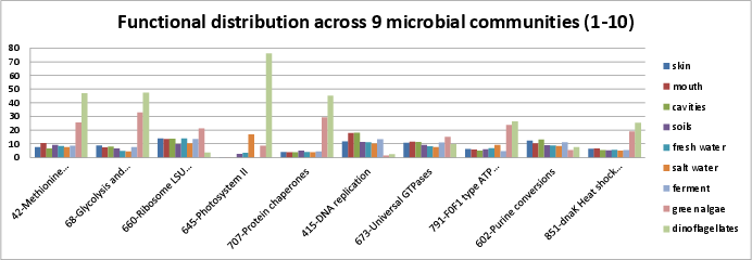
The ten most prevalent categories include:
si_0042; Methionine biosynthesisin the Amino Acids and Derivatives rollup category. It can be found on Kegg map 270. The SEED description by Dmitry Rodionov describes a variet of pathways leading to methionine.si_0068; Glycolysis and Gluconeogenesisin the Carbohydrates rollup category. It can be found on Kegg map 10. The SEED description by Svetlana Gerdes and Ross Overbeek, describe glycolysis and gluconeogenesis.si_0660; Ribosome LSU bacterialin the Protein Metabolism rollup category. It can be found on Kegg map 3010.si_0645; Photosystem IIin the Photosynthesis rollup category. It can be found on Kegg map 195.si_0707; Protein chaperonesin the Protein Metabolism rollup category. DnaJ is HSP-40 and dnaK is HSP-70. See the Wikipedia page and PMID 16952052.si_0415; DNA replicationin the DNA Metabolism rollup category.si_0673; Universal GTPasesin the Protein Metabolism rollup category. Caldon, et al. suggest that the 11 universal GTPases are either necessary for ribosome function or transmitting information from the ribosome to downstream targets for the purpose of generating specific cellular responses.si_0791; F0F1 type ATP synthasein the Respiration rollup category. It can be found on Kegg map 195.si_0602; Purine conversionsin the Nucleosides and Nucleotides rollup category. It can be found on Kegg map 230.si_0851; dnaK Heat shock clusterin the Stress Response rollup category. DnaJ is HSP-40 and dnaK is HSP-70. See the Wikipedia page and PMID 16952052.
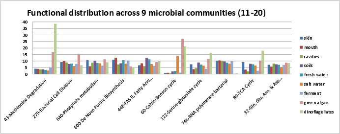
Categories 11-20 include:
si_0043; Methionine Degradationin the Amino Acids and Derivatives rollup category. It can be found on Kegg map 270si_0279; Bacterial Cell Divisionin the Clustering-based subsystems rollup category. It can be found on Kegg map 4112.si_0640; Phosphate metabolismin the Phosphorous Metabolism rollup category. Some description can be found in Gebhard, et al..si_0600; De Novo Purine Biosynthesisin the Nucleosides and Nucleotides rollup category. It can be found on Kegg map 230.si_0448; FAS II; Fatty Acid Biosynthesisin the Fatty Acids, Lipids, and Isoprenoids rollup category. It can be found on Kegg map 61 for biosynthesis, Kegg map 62 for elongation. The SEED description by Andrei Osterman describes fatty acid biosynthesis through FAS II, which is largely homologous to FAS I.si_0060; Calvin-Benson cyclein the Carbohydrates rollup category. It can be found on Kegg map 710.si_0122; Serine-glyoxylate cyclein the Carbohydrates rollup category. It can be found on Kegg map 630.si_0746; RNA polymerase bacterialin the RNA Metabolism rollup category. It can be found on Kegg map 3020.si_0080; TCA Cyclein the Carbohydrates rollup category. It can be found on Kegg map 20.si_0032; Gln, Glu, Asn, & Asp Biosynthesisin the Amino Acids and Derivatives rollup category. It can be found on Kegg map 250.
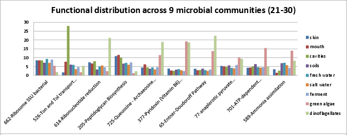
Categories 21-30 include:
si_0662; Ribosome SSU bacterialin the Protein Metabolism rollup category. It can be found on Kegg map 3010.si_0526; Ton and Tol transport systemsin the Membrane Transport rollup category. Danese, et al. describe the Ton system to obtain iron in Brucella spp. Housden, et al. describe how Ton and Tol facilitate uptake of chelated iron or group B colicins through active transport.si_0614; Ribonucleotide reductionin the Nucleosides and Nucleotides rollup category. The Wikipedia article describes how ribonucleotide reductase converts RNA to DNA, maintaining an appropriate concentration of DNA throughout the cell cycle. The SEED description by Dmitry Rodinov desribes the three classes of ribonucleotide reductases.si_0205; Peptidoglycan Biosynthesisin the Cell Wall and Capsule rollup category. It can be found on Kegg map 550. The SEED description by Vassily Portnoy, Olga Vassieva, and Rick Stevens describes peptidoglycan biosynthesis.si_0725; Queuosine - Archaeosine Biosynthesisin the RNA Metabolism rollup category. The SEED description describes the synthesis and incorporation of the modified bases of tRNA, Queuosine and Archaeosine.si_0377; Pyridoxin (Vitamin B6) Biosynthesisin the Cofactors, Vitamins, Prosthetic Groups, Pigments rollup category. It can be found on Kegg map 750.si_0065; Entner-Doudoroff Pathwayin the Carbohydrates rollup category. From Wikipedia, the Entner-Doudoroff pathway is a low-efficiency pathway to take glucose to pyruvate, found mostly in Gram-negative organisms, such as Pseudomonas, Rhizobium, Azotobacter, and Agrobacterium.si_0077; anaplerotic pyruvate metabolism I: PEPin the Carbohydrates rollup category. It can be found on Kegg map 20. See the Wikipedia article.si_0701; ATP-dependent proteolysis in bacteriain the Protein Metabolism rollup category.si_0589; Ammonia assimilationin the Nitrogen Metabolism rollup category. It can be found on Kegg map 910. The SEED description by Ed Frank, describes the glutamate dehydrogenase or GS-GOGAT pathways.
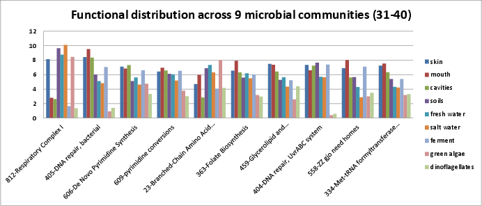
Categories 31-40 include:
si_0812; Respiratory Complex Iin the Respiration rollup category.si_0405; DNA repair, bacterialin the DNA Metabolism rollup category. The SEED description by Michael Kubal, describes a process of DNA base excision repair through detection, breakage, exonuclease activity, DNA polyerase, and DNA ligase.si_0606; De Novo Pyrimidine Synthesisin the Nucleosides and Nucleotides rollup category. It can be found on Kegg map 240.si_0609; pyrimidine conversionsin the Nucleosides and Nucleotides rollup category. It can be found on Kegg map 240.si_0023; Branched-Chain Amino Acid Biosynthesisin the Amino Acids and Derivatives rollup category. It can be found on Kegg map 290.si_0363; Folate Biosynthesisin the Cofactors, Vitamins, Prosthetic Groups, Pigments rollup category. It can be found on Kegg map 790. The SEED description by Valerie de Crecy-Lagard and Andrew Hanson describes folate biosynthesis.si_0459; Glycerolipid and Glycerophospholipid Metabolismin the Fatty Acids, Lipids, and Isoprenoids rollup category. It can be found on Kegg map 561 and Kegg map 564. The SEED description by Vasiliy Portnoy describes glycerolipid an diglycerophospholipid biosynthesis.si_0404; DNA repair, UvrABC systemin the DNA Metabolism rollup category.si_0558; ZZ gjo need homesin the Miscellaneous rollup category.si_0334; Met-tRNA formyltransferase gene clusterin the Clustering-based subsystems rollup category.
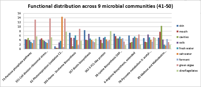
Categories 41-50 include:
si_0073; Pentose phosphate pathwayin the Carbohydrates rollup category. It can be found on Kegg map 30.si_0331; Cell division-ribosomal stress proteins clusterin the Clustering-based subsystems rollup category.si_0062; Photorespiration (oxidative C2 cycle)in the Carbohydrates rollup category.si_0393; Heme - Siroheme Biosynthesisin the Cofactors, Vitamins, Prosthetic Groups, Pigments rollup category. It can be found on Kegg map 860. The SEED description by Svetlana Gerdes describes tetrapyrrole biosynthesis.si_0357; Biotin biosynthesisin the Cofactors, Vitamins, Prosthetic Groups, Pigments rollup category. It can be found on Kegg map 780. The SEED description by Dmitry Rodionov, describes how biotin, vitamin H, which is an essential cofactor for a class of important metabolic enzymes.si_0362; 5-FCL-like proteinin the Cofactors, Vitamins, Prosthetic Groups, Pigments rollup category.si_0038; Lysine Biosynthesis DAP Pathwayin the Amino Acids and Derivatives rollup category. It can be found on Kegg map 300.si_0006; Arginine Biosynthesis, extendedin the Amino Acids and Derivatives rollup category. It can be found on Kegg map 330.si_0078; Pyruvate metabolism II: acetyl-CoA, acetogenesis from pyruvatein the Carbohydrates rollup category. It can be found on Kegg map 620 and Kegg map 770.si_0085; Maltose and Maltodextrin Utilizationin the Carbohydrates rollup category. It can be found on Kegg map 500.

Categories 51-60 include:
si_0059; CO2 uptake, carboxysomein the Carbohydrates rollup category.si_0654; Potassium homeostasisin the Potassium metabolism rollup category.si_0002; Glycine and Serine Utilizationin the Amino Acids and Derivatives rollup category. It can be found on Kegg map 260.si_0668; Translation elongation factors bacterialin the Protein Metabolism rollup category.si_0455; Isoprenoid Biosynthesisin the Fatty Acids, Lipids, and Isoprenoids rollup category. The SEED description by Olga Zagnitko, describes how the major terpenoid building blocks, isopentenyl diphosphate and dimethylallyl diphosphate, are produced by the mevalonate and non-mevalonate pathways.si_0178; Sialic Acid Metabolismin the Cell Wall and Capsule rollup category.si_0135; Glycogen metabolismin the Carbohydrates rollup category. It can be found on Kegg map 500.si_0153; Bacterial Cytoskeletonin the Cell Division and Cell Cycle rollup category.si_0046; Threonine and Homoserine Biosynthesisin the Amino Acids and Derivatives rollup category. It can be found on Kegg map 260.si_0403; DNA Repair; Base Excisionin the DNA Metabolism rollup category.
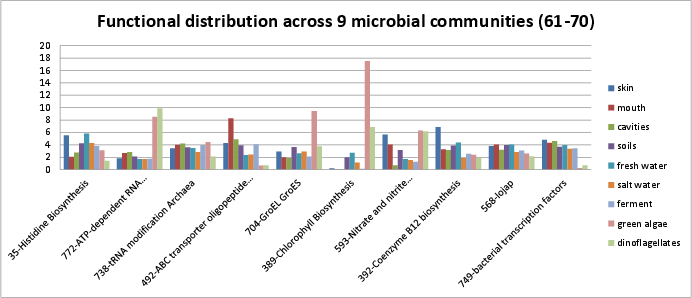
Categories 61-70 include:
si_0035; Histidine Biosynthesisin the Amino Acids and Derivatives rollup category. It can be found on Kegg map 340.si_0772; ATP-dependent RNA helicases, bacterialin the RNA Metabolism rollup category.si_0738; tRNA modification Archaeain the RNA Metabolism rollup category.si_0492; ABC transporter oligopeptide (TC_3.A.1.5.1)in the Membrane Transport rollup category.si_0704; GroEL GroESin the Protein Metabolism rollup category.si_0389; Chlorophyll Biosynthesisin the Cofactors, Vitamins, Prosthetic Groups, Pigments rollup category. It can be found on Kegg map 860. The SEED description by Svetlana Gerdes and Veronika Vonstein, describes the biosynthesis of chlorophyll, used in photosynthesis.si_0593; Nitrate and nitrite ammonificationin the Nitrogen Metabolism rollup category. It can be found on Kegg map 910.si_0392; Coenzyme B12 biosynthesisin the Cofactors, Vitamins, Prosthetic Groups, Pigments rollup category.si_0568; Iojapin the Miscellaneous rollup category.si_0749; bacterial transcription factorsin the RNA Metabolism rollup category.
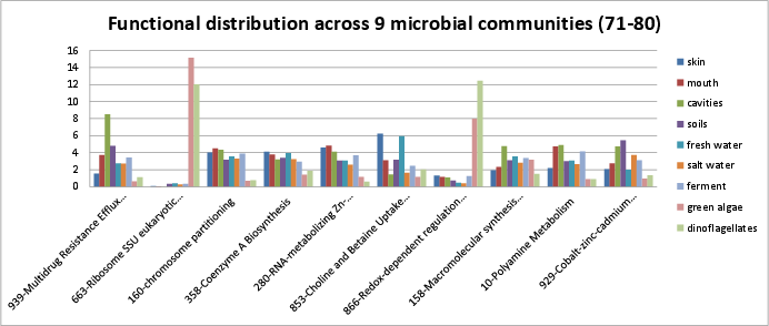
Categories 71-80 include:
si_0939; Multidrug Resistance Efflux Pumpsin the Virulence, Disease, and Defense rollup category.si_0663; Ribosome SSU eukaryotic and archaealin the Protein Metabolism rollup category.si_0160; chromosome partitioningin the Cell Division and Cell Cycle rollup category.si_0358; Coenzyme A Biosynthesisin the Cofactors, Vitamins, Prosthetic Groups, Pigments rollup category. It can be found on Kegg map 770.si_0280; RNA-metabolizing Zn-dependent hydrolasesin the Clustering-based subsystems rollup category.si_0853; Choline and Betaine Uptake and Betaine Biosynthesisin the Stress Response rollup category.si_0866; Redox-dependent regulation of nucleus processesin the Stress Response rollup category.si_0158; Macromolecular synthesis operonin the Cell Division and Cell Cycle rollup category.si_0010; Polyamine Metabolismin the Amino Acids and Derivatives rollup category.si_0929; Cobalt-zinc-cadmium resistancein the Virulence, Disease, and Defense rollup category.
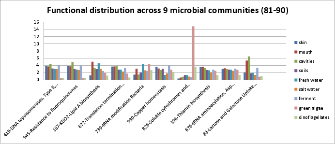
Categories 81-90 include:
si_0419; DNA topoisomerases, Type II, ATP-dependentin the DNA Metabolism rollup category. They are described in the Wikipedia article.si_0945; Resistance to fluoroquinolonesin the Virulence, Disease, and Defense rollup category. Fluoroquinolones target DNA gyrase and topoisomerase IV. See Hooper, et al..si_0187; KDO2-Lipid A biosynthesisin the Cell Wall and Capsule rollup category.si_0672; Translation termination factors bacterialin the Protein Metabolism rollup category.si_0739; tRNA modification Bacteriain the RNA Metabolism rollup category.si_0930; Copper homeostasisin the Virulence, Disease, and Defense rollup category.si_0826; Soluble cytochromes and functionally related electron carriersin the Respiration rollup category.si_0396; Thiamin biosynthesisin the Cofactors, Vitamins, Prosthetic Groups, Pigments rollup category. The SEED description by Dmitry Rodionov describes how vitamin B1, thiamin, is synthesized.si_0676; tRNA aminoacylation, Asp and Asnin the Protein Metabolism rollup category.si_0083; Lactose and Galactose Uptake and Utilizationin the Carbohydrates rollup category. It can be found on Kegg map 052.
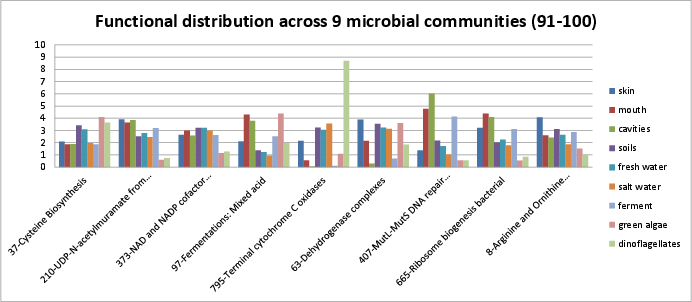
Categories 91-100 include:
si_0037; Cysteine Biosynthesisin the Amino Acids and Derivatives rollup category. It can be found on Kegg map 270.si_0210; UDP-N-acetylmuramate from Fructose-6-phosphate Biosynthesisin the Cell Wall and Capsule rollup category. The SEED description by Vasiliy Portnoy and Olga Zagnitko describes production of a major building block for biosynthesis of peptidoglycan.si_0373; NAD and NADP cofactor biosynthesis ,globalin the Cofactors, Vitamins, Prosthetic Groups, Pigments rollup category. The SEED description by Andrei Osterman describes NAD and NADP biosynthesis.si_0097; Fermentations: Mixed acidin the Carbohydrates rollup category.si_0795; Terminal cytochrome C oxidasesin the Respiration rollup category. It can be found on Kegg map 190.si_0063; Dehydrogenase complexesin the Carbohydrates rollup category.si_0407; MutL-MutS DNA repair system, bacterialin the DNA Metabolism rollup category. It can be found on Kegg map ko03430.si_0665; Ribosome biogenesis bacterialin the Protein Metabolism rollup category.si_0008; Arginine and Ornithine Degradationin the Amino Acids and Derivatives rollup category. It can be found on Kegg map 330.
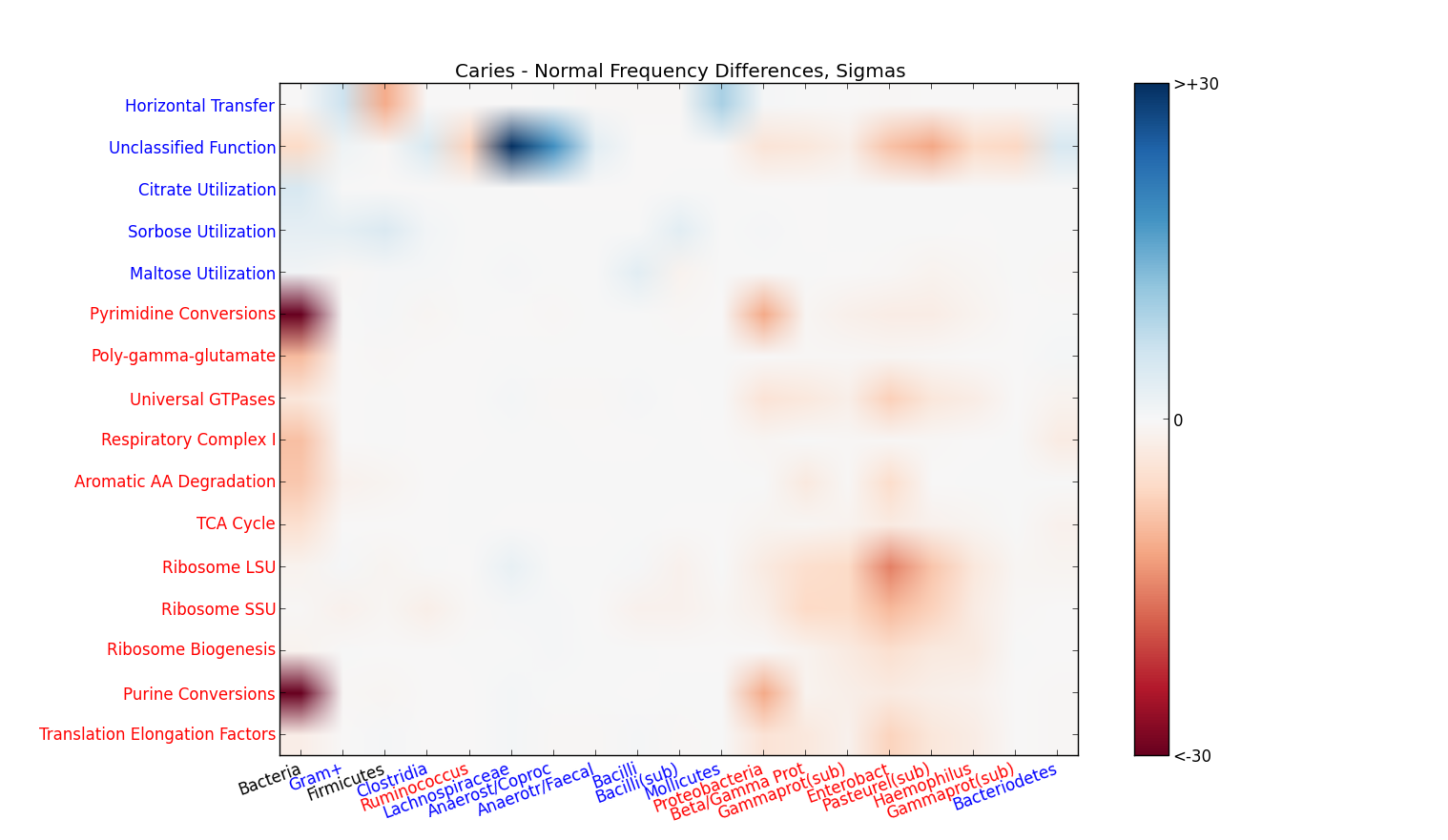
7.3. Identifying enriched functions
Using field replicates to identify important determinants of ecosystem function
face figure
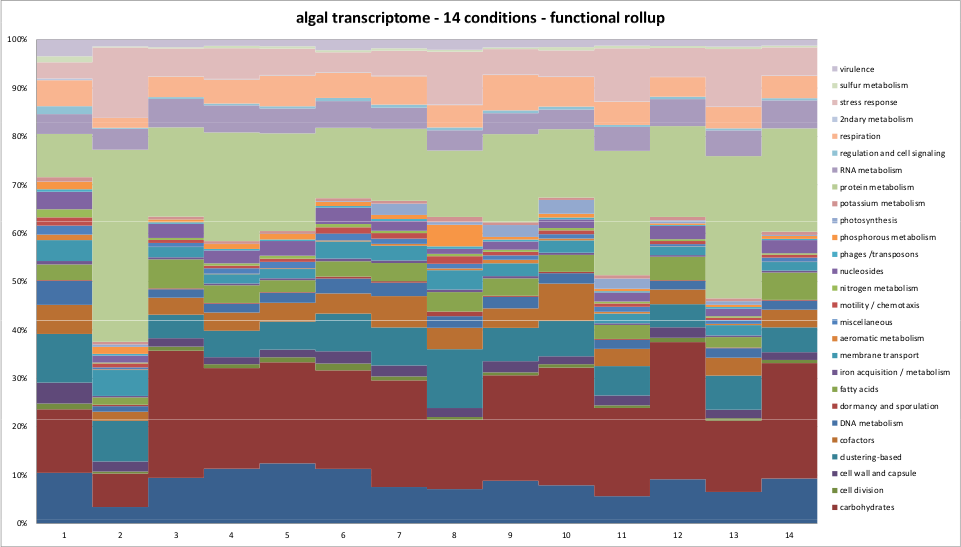
Algal transcriptomes
Tooth decay study