6. Using Sequestat
Sequestat is a suite of functions and visualizations written for analysis of Sequedex output in the statistical visualization package, R. Installation instructions and hints to getting started with R are provided in Statistical analysis and graphing with R and R Studio. RStudio provides a graphical environment with pull-down menus and more convenient ways to perform many tasks, but we provide instructions for the simpler, terminal window, interface to R. These instructions will work in both R and Rstudio.
The easiest way to get started with Sequestat in R is to first download
sequestat.r and the nexus-format phylogenetic
tree used with the Life2550 data modules Life2550.nexus and then examine sets of already-compiled output files
from three large data sets:
- the set of
synthetic data from reference genomeswithlabels, - a set of
environmental microbiomeswithlabels - a set of
human microbiomeswithlabels
Readers who have aready analyzed data sets, and have the Sequedex output files available on their desktop computers can skip ahead to Reading Life2550 output files into Sequestat: or Reading virus1252 output files into Sequestat:.
6.1. Visualizing phylogenetic data with Sequestat
Once R or Rstudio is started, the human microbiome data can be loaded into R or Rstudio and plotted with the commands:
source("~/Sequedex-docs/dl/sequestat.r")

filename="~/Sequedex-docs/dl/hmb.Life.who"
labelfile="~/Sequedex-docs/dl/hmb.Life.lbl"

dat=read.table(filename,header=F,sep="\t")
lab=read.table(labelfile,header=F,sep="\t")
lab=lab[!is.na(lab)]
nn=dim(dat)[1]-1
rname=c(paste("n000",0:9,sep=""),paste("n00",10:99,sep=""),paste("n0",100:999,sep=""),paste("n",1000:nn,sep=""))
colnames(dat)=lab
rownames(dat)=rname
A set of PDF files that together tile the entire tree, Life2550, are available at _s.Life2550, above each of the sections, with node numbers, family, phylum, and taxon names. Sub-trees can then be viewed in R by typing the following:
Plot.profile(expts,1,"n0000",tip.frq=1,use.edge.length=T,type="phylo",show.tip.label=T)
where “n0000” is the node number defining the subtree to be plotted.
The node number that is the second argument of the above function call
is defined by the phyloxml file,
that can be viewed with archaeopteryx, as described in Exploring trees with Archaeoptrix, FigTree, or NJPlot.
Alternatively, section Tree of Life, 2550 taxa contains node numbers for a
variety of families and phyla, and 23 pdf files detailing a spanning
set of subtrees. To define subtrees by label in a way that covers the
categories included in the high level rollup categories for the tree
Life2550, copy the following lines into your R session:
root="n0000"; bacteria="n0001"; gramp="n1220"; gramn="n0002"; euks="n2401"; metazoa="n2447"; fungi="n2482"; protozoa="n2402"
archaea="n2214"; crenarch="n2218"; euryarch="n2259"
elusi="n0005";fuso="n0008"; spiro="n00025"; chlamydia="n0075"; chlorobi="n0115"; bacteroidetes="n0127"
adeprot="n0301"; eprot="n0302"; aquificae="n0342"; acidobacteria="n0354"; dprot="n0369"; aprot="n0429"
rhiz="n0596"; rhodo="n0536"; sphingo="n0509"; rhodospirillaceae="n0470"; rickettsiales="n0430"
bgprot="n0691"; gprot="n0692"; enteric="n0705"; pasteurellales="n0793"; vibrio="n0818"; shewanella="n0860";
altero="n0879"; gprot2="n0912"; moraxellaceae="n0980"; xanthomonads="n1011"; francisella="n1072";
bprot="n1083"; burk="n1086"; neisseria="n1197"; nitrosomonas="n1183"
actino="n1221"; coriobacteriales="n1222"; actinomyces="n1244"; streptomyces="n1334"; nocardia="n1387"; frankia="n1374"
chloroflexi="n1572";deino="n1512"; clostridia="n1591";negativicutes="n1784"; peptococcaceae="n1758";
clostridia="n1596";clostridia1="n1601";ruminococcus="n1650";thermoanaero="n1679"
lactobacillales="n1822";strep="n1826"; lactobacillaceae="n1875"
cyano="n2120";plasmas="n2065";staph="n1958";bacillus="n1988";paenibacillaceae="n2041";bacillales="n1957"
The abbreviations are somewhat arbitrary, with groups sometimes matching families or phyla, and sometimes more of a pneumonic; it is easy for the user to define his or her own families and labels. Once defined, however, the beta proteobacteria portion of the tree can be seen with the command:
Plot.profile(expts,1,bprot,tip.frq=1,use.edge.length=T,type="phylo",show.tip.label=T)
If you type the command:
expts$data[0,]
you will see the labels of the individual columns of data who’s phylogenetic profiles are available in this session, and if you type ls(), you will see the list of defined functions and variables.
The user is invited to explore the full phylogenetic extent and plotting options available to this function by altering the various arguments to the Plot.profile function.
hmb <- Read.tree(“~/Sequedex-docs/dl/Life2550.nexus”) hmb$data <- dat hmb$node.label <- rname
hmb$data[0,] #list sample labels in order of column number
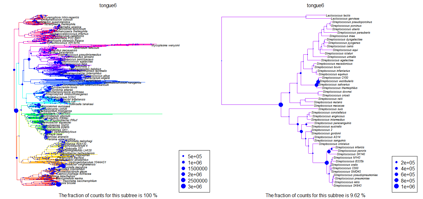
Plot.profile(hmb,”tongue6”,”n0000”,tip.frq=25,use.edge.length=T,type=”phylo”) Plot.profile(hmb,”tongue6”,strep,tip.frq=25,use.edge.length=T,type=”phylo”)
results in figures like the following
This data set can be explored as above. Similarly, the environmental data can be loaded with the commands:
filename="~/Sequedex-docs/dl/env.Life.who"
labelfile="~/Sequedex-docs/dl/env.Life.lbl"
dat=read.table(filename,header=F,sep="\t")
lab=read.table(labelfile,header=F,sep="\t")
lab=lab[!is.na(lab)]
nn=dim(dat)[1]-1
rname=c(paste("n000",0:9,sep=""),paste("n00",10:99,sep=""),paste("n0",100:999,sep=""),paste("n",1000:nn,sep=""))
colnames(dat)=lab
rownames(dat)=rname
env <- Read.tree("Life2550.nexus")
env$data <- dat
env$node.label <- rname
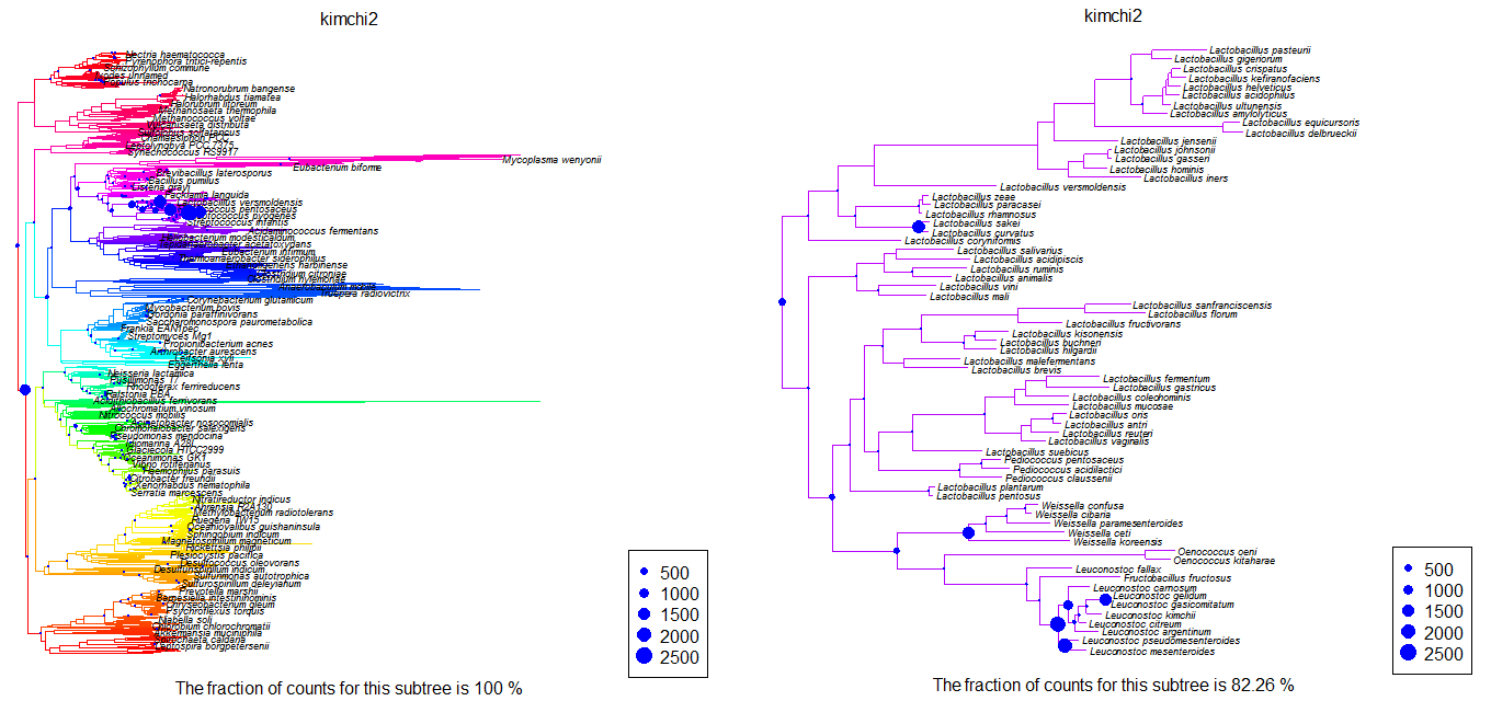
Plot.profile(env,"kimchi2",root,tip.frq=25,use.edge.length=T,type="phylo")
Plot.profile(env,"kimchi2","n1875",tip.frq=25,use.edge.length=T,type="phylo")
produces plots like
and the synthetic data evaluation with:
filename="~/Sequedex-docx/dl/syn.Life.who"
labelfile="~/Sequedex-docx/dl/syn.Life.lbl"
dat=read.table(filename,header=F,sep="\t")
lab=read.table(labelfile,header=F,sep="\t")
lab=lab[!is.na(lab)]
nn=dim(dat)[1]-1
rname=c(paste("n000",0:9,sep=""),paste("n00",10:99,sep=""),paste("n0",100:999,sep=""),paste("n",1000:nn,sep=""))
colnames(dat)=lab
rownames(dat)=rname
syn <- Read.tree("~/Sequedex-docx/dl/Life2550.nexus")
syn$data <- dat
syn$node.label <- rname
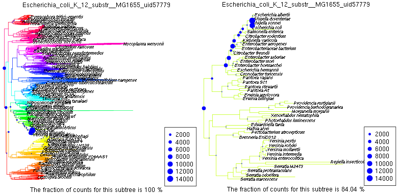
Plot.profile(syn,"Escherichia_coli_K_12_substr__MG1655_uid57779","n0000",tip.frq=35,use.edge.length=T,type="phylo")
Plot.profile(syn,"Escherichia_coli_K_12_substr__MG1655_uid57779","n0707",tip.frq=2,use.edge.length=T,type="phylo")
produces plots like
These data sets can all be explored using the node numbers defined in Tree of Life, 2550 taxa or the phylogenetic groupings defined above, once the definitions are pasted into R. We assume the field separator in the read.table command needs to match the one in the input file.
6.2. Reading Life2550 output files into Sequestat:
To read in his or her own data from a set of directories of Sequestat output files, assumed to subdirectories of ~/expts/., with sequestat.r and the reference tree, Life2550.nexus in ~/Sequedex-docs/dl/, as described at the beginning of Getting started, a user should type:
source("~/Sequedex-docs/dl/sequestat.r")
expts=Read.phylo("~/expts","./Life2550.nexus")
Plot.profile(expts,1,"n0000",tip.frq=30,use.edge.length=T,type="phylo",show.tip.label=T)
at the R or Rstudio command prompt. At this point, a plot of the entire 2550 taxa tree of life should appear on the screen, with dots on the nodes indicating the number of reads in data set 3 assigned to each node. It is likely that the use will want to make trees of specific families. Plot.profile, which will display Sequedex output on either the entire reference tree, or of a subtree defined by a node number on the overall tree:
Plot.profile(expts,3,"n0000",use.edge.length=T,type="unrooted",show.tip.label=F)
6.3. Reading virus1252 output files into Sequestat:
When viewing output from the virus1252 data module wiht Sequestat in
R, once again, source sequestat.r but
dl/virus1252.nexus read in a set of
directories of Sequestat output files, assumed to subdirectories of
~/expts/., with sequestat.r and the reference tree, virus1252.nexus in
the working directory of R:
source("~/Sequedex-docs/dl/sequestat.r")
expts=Read.phylo("~/vexpts","~/Sequedex-docs/dl/virus1252.nexus")
Plot.profile(vexpts,1,"n0000",tip.frq=30,use.edge.length=T,type="phylo",show.tip.label=T)
At this point, a plot of the entire 1252 taxa viral tree should appear on the screen, with dots on the nodes indicating the number of reads in data set 3 assigned to each node. It is likely that the use will want to make trees of specific families. Plot.profile which will display Sequedex output on either the entire reference tree, or of a subtree defined by a node number on the overall tree:
Plot.profile(vexpts,3,"n0000",use.edge.length=T,type="unrooted",show.tip.label=F)
Sub-trees can then be viewed in R by typing the following:
Plot.profile(vexpts,1,"n0000",tip.frq=1,use.edge.length=T,type="phylo",show.tip.label=T)
where “n0000” is the node number defining the subtree to be plotted.
The node number that is the second argument of the above function call
is defined on the phyloxml tree dl/virus1252.phyloxml,
that can be viewed with archaeopteryx, as described in Exploring trees with Archaeoptrix, FigTree, or NJPlot.
Alternatively, section Viral tree, 1252 taxa contains node numbers for a
variety of families and phyla, and 17 png image files detailing a
spanning set of subtrees. To define subtrees by label in a way that
covers the categories included in the high level rollup categories for
the tree Life2550, copy the following lines into your R session:
root=0; dsDNA=1; dsDNA1=3; Baculo=5; Phycodna=51; Irido=63
dsDNA2=70; Papilloma=71; Polyoma=144; Pox=162
dsDNA3=180; Adeno=181; Herpes=215
RT=263; Caulimo=264; Retro=297; Hepadna=338
ssRNAp1=345; Calici=346; Nido=363
ssRNAp2=395; Flavi=395; Flavi1=396; Flavi2=432
ssRNAp2345=394; Tombus=446; Virga=470
ssRNAp4=503; Tymo=503; Tymo1=505; Tymo2=552; Tymo3=594
ssRNAp5=605; Picorna=606; Picorna1=608; Picorna2=687; Picorna3=714; Toga=721
ssRNAp6=735; Poty=735; Poty1=736; Poty2=805
ssRNAm=816; segRNAm=817; Arena=818; Bunya=843
Mononega=865; Mononega1=866; Mononega2=904;
Orthomyxo=931
ssDNA1=949; Parvo=949
ssDNA23=987; Gemini1=988; Gemini2=1230
dsDNA=1253; Reo=1253
The abbreviations are somewhat arbitrary, with groups sometimes matching families or phyla, and sometimes more of a pneumonic; it is easy for the user to define his or her own families and labels. Once defined, however, the beta proteobacteria portion of the tree can be seen with the command:
Plot.profile(expts,1,bprot,tip.frq=1,use.edge.length=T,type="phylo",show.tip.label=T)
If you type the command:
expts$data[0,]
you will see the labels of the individual columns of data who’s phylogenetic profiles are available in this session, and if you type ls(), you will see the list of defined functions and variables.
The user is invited to explore the full phylogenetic extent and plotting options available to this function by altering the various arguments to the Plot.profile function.
6.4. Decomposing mixture into components with Sequestat
Even complex metagenomic samples often have dominant organisms, and when they are phylogenetically close to organisms in the reference database, the distiribution of reads across the nodes of the tree, above, can be used to identify what organisms are present. If this process identifies something closely related to an organism of particular interest to the user, follup analysis should be performed, as described in Annotated reads.
The strategy for decomposing the metagenomic phylogenetic profile into a mixture is to create a synthetic data set for the broadest possible array of curated organisms, thin this list, run Sequedex on this synthetic data with a particular tree (and ideally identical signature list), cluster this list, then fit the unknown sample to a linear combination of reference profiles.
- step 1: clean the raw profiles by removing profiles that either have less than 1000 hits (mainly divergent organisms) or profiles that have over 7.5% of reads that are not monophyletic (possibly contaminated organisms)
- step 2: cluster the remainin profiles into 800 groups
- step 3: use the lasso to model the normalized metagenomic profile asa linear combination of cluster profiles. Use only nodes that are at depth 4 or less from the leaves
- step 4: extract the top 100 clusters (use RSS to assess if this number is too small) that list is an upper bound of the possible profiles
- step 5: Use traditional model selection approach to select significant profiles (use k=1.25 be more inclusive than AIC)
Starting a new session in R or RStudio, and download
demo_protocol.r,
syn.Life.who, syn.Life.lbl Life2550.nexus into
your working directory. Start R or RStudio in this directory and
type:
source("~/Sequedex-docx/dl/demo_protocol.r")
Sequestat will chug along for a few minutes to completion. Typing sig.list will result in:
> sig.list
$`V202 0.31281`
[1] "Staphylococcus_caprae_C87_uid61125"
[2] "Staphylococcus_epidermidis_ATCC_12228_uid57861"
[3] "Staphylococcus_warneri_SG1_uid187059"
[4] "Staphylococcus_aureus_04_02981_uid161969"

$`V66 0.24039`
[1] "Sphingobium_SYK_6_uid73353"
[2] "Zymomonas_mobilis_ATCC_10988_uid55403"
[3] "Sphingomonas_wittichii_RW1_uid58691"
[4] "Sphingomonas_KC8_uid77733"
[5] "Sphingomonas_elodea_ATCC_31461_uid157063"
[6] "Sphingomonas_S17_uid66923"

$`V368 0.11183`
[1] "Novosphingobium_aromaticivorans_DSM_12444_uid57747"
[2] "Novosphingobium_nitrogenifigens_DSM_19370_uid64475"
[3] "Sphingomonas_LH128_uid174245"
[4] "Novosphingobium_AP12_uid171681"
[5] "Novosphingobium_Rr_2_17_uid170038"

$`V742 0.08731`
[1] "Staphylococcus_pettenkoferi_VCU012_uid179999"
[2] "Staphylococcus_arlettae_CVD059_uid175126"

$`V490 0.06027`
[1] "Staphylococcus_hominis_C80_uid61127"
[2] "Staphylococcus_haemolyticus_JCSC1435_uid62919"

$`V584 0.05848`
[1] "Staphylococcus_lugdunensis_HKU09_01_uid46233"

$`V420 0.04302`
[1] "Bacteroides_vulgatus_ATCC_8482_uid58253"
[2] "Bacteroides_plebeius_DSM_17135_uid54991"
[3] "Bacteroides_coprophilus_DSM_18228_uid55301"
[4] "Bacteroides_salanitronis_DSM_18170_uid63269"
[5] "Bacteroides_coprocola_DSM_17136_uid54879"

$`V821 0.03858`
[1] "Bacteroides_ovatus_3_8_47FAA_uid68195"
[2] "Bacteroides_xylanisolvens_CL03T12C04_uid181622"

$`V920 0.0318`
[1] "Staphylococcus_pseudintermedius_ED99_uid162109"

$`V790 0.02675`
[1] "Erythrobacter_NAP1_uid54197"
[2] "Erythrobacter_litoralis_HTCC2594_uid58299"
[3] "Erythrobacter_SD_21_uid54677"

$`V848 0.02402`
[1] "Bacteroides_finegoldii_CL09T03C10_uid181638"
[2] "Bacteroides_caccae_ATCC_43185_uid54521"
[3] "Bacteroides_faecis_MAJ27_uid86875"

$`V192 0.01953`
[1] "Macrococcus_caseolyticus_JCSC5402_uid59003"
[2] "Sporosarcina_newyorkensis_uid70561"
[3] "Solibacillus_silvestris_StLB046_uid168516"
[4] "Listeria_grayi_DSM_20601_uid55523"

$`V712 0.01661`
[1] "Staphylococcus_carnosus_TM300_uid59401"

$`V761 0.00867`
[1] "Novosphingobium_pentaromativorans_US6_1_uid78315"
[2] "Novosphingobium_PP1Y_uid67383"

$`V774 0.00743`
[1] "Sphingomonas_SKA58_uid54251"

$`V539 -0.02038`
[1] "Rhodospirillum_centenum_SW_uid58805"
[2] "Oceanibaculum_indicum_P24_uid176351"
[3] "Thalassobaculum_L2_uid182483"
[4] "SAR_116_cluster_alpha_proteobacterium_HIMB100_uid78325"
[5] "Candidatus_Puniceispirillum_marinum_IMCC1322_uid47081"

$`V985 -0.02118`
[1] "Phenylobacterium_zucineum_HLK1_uid58959"

$`V475 -0.03216`
[1] "Sphingopyxis_alaskensis_RB2256_uid58351"

$`V710 -0.05337`
[1] "Parvularcula_bermudensis_HTCC2503_uid51641"
[2] "Hirschia_baltica_ATCC_49814_uid59365"
[3] "Hyphomonas_neptunium_ATCC_15444_uid58433"
[4] "Parvibaculum_lavamentivorans_DS_1_uid58739"
Typing mGlbl will list the metagenomic samples loaded into this list, with the top portion of the output shown here:
> mGlbl
[1] "nose1"        "nose2"        "nose3"        "nose4"        "nose5"
[6] "nose6"        "nose7"        "nose8"        "nose9"        "nose10"
[11] "nose11"       "nose12"       "nose13"       "nose14"       "nose15"
[16] "nose16"       "nose17"       "nose18"       "nose19"       "nose20"
[21] "nose21"       "nose22"       "nose23"       "nose24"       "nose25"
[26] "nose26"       "nose27"       "nose28"       "nose29"       "nose30"
[31] "nose31"       "nose32"       "nose33"       "nose34"       "nose35"
[36] "nose36"       "nose37"       "nose38"       "nose39"       "nose40"
[41] "nose41"       "nose42"       "nose43"       "nose44"       "nose45"
[46] "nose46"       "nose47"       "nose48"       "nose49"       "nose50"
[51] "nose51"       "nose52"       "nose53"       "nose54"       "nose55"
[56] "nose56"       "nose57"       "nose58"       "nose59"       "nose60"
[61] "nose61"       "nose62"       "nose63"       "nose64"       "nose65"
[66] "nose66"       "nose67"       "nose68"       "nose69"       "nose70"
[71] "nose71"       "nose72"       "nose73"       "nose74"       "nose75"
[76] "nose76"       "nose77"       "nose78"       "nose79"       "nose80"
[81] "nose81"       "nose82"       "nose83"       "nose84"       "nose85"
[86] "nose86"       "nose87"       "nose88"       "nose89"       "l.ear1"
[91] "l.ear2"       "l.ear3"       "l.ear4"       "l.ear5"       "l.ear6"
[96] "l.ear7"       "l.ear8"       "r.ear1"       "r.ear2"       "r.ear3"
[101] "r.ear4"       "r.ear5"       "r.ear6"       "r.ear7"       "r.ear8"
[106] "r.ear9"       "r.ear10"      "r.ear11"      "r.ear12"      "r.ear13"
[111] "r.ear14"      "r.ear15"      "r.ear16"      "r.ear17"      "r.ear18"
[116] "tongue1"      "tongue2"      "tongue3"      "tongue4"      "tongue5"
To profile a different sample, simply re-run the last part of the demo_protocol.r code, with a new value for meta.idx. If you have labels defined, the command meta.idx = match(“stool1”,mGlbl) will select the correct column on the basis of the label. If you associate the tabular data with a tree, a described in s.read.sequedex or s.sets, you can compare the node plots to the lists of possible taxa. Here is the last part of the demo_protocol code, for cutting and pasting:
#=========================================================
#  apply algorithm to a selected metagenome

meta.idx <- 1
#meta.idx = match("stool1",mGlbl)

Y0 <- metaG[,meta.idx]/sum(metaG[,meta.idx])
Y0 <- Y0[ndepth < 251 ]
fit0 <- lars(PP,Y0,type="lasso",intercept=F,normalize=F,max.steps=300,use.Gram=F)

#--------------------------------------------------------
#  step 4: extract the top 100 clusters

nvar <- 200
idx <- max((1:length(fit0$df))[fit0$df <= nvar])
rss <- fit0$RSS
bb <- fit0$beta[idx,]
cc <- bb[bb != 0]
big.list <- cc.name[bb != 0]
big.list <- big.list[sort.list(bb[bb != 0],decreasing=T)]

#-----------------------------------------------------------
#  step 5: Use traditional model selection approach to select significant profiles

vnames <- paste("V",1:dim(PP)[2],sep="")
colnames(PP) <- vnames
names(cc.name) <- vnames
mnames <- vnames[bb != 0]
mmodel0 <- formula(paste("Y0 ~ 0 + ",mnames[1]))
mmodel1 <- formula(paste("Y0 ~ ",paste(mnames,collapse=" + ")))
fit1 <- lm( mmodel0 ,data=as.data.frame(PP))
fit2 <- step(fit1, mmodel1, data=as.data.frame(PP),k=2)

sig.list <- cc.name[(names(fit2$coef))]
sig.list <- sig.list[sort.list(fit2$coef,decreasing=T)]
names(sig.list) <- paste(names(sig.list),sort(round(fit2$coef,5),decreasing=T))